

Imagine you are building a Discounted Cash Flow (DCF) model for a high-growth tech company or a stable infrastructure asset. You meticulously forecast every line item for the next five years: revenue growth, EBITDA margins, working capital, and CapEx. You arrive at your Unlevered Free Cash Flows ($UFCF$), discount them using the WACC, and sum them up.
Then comes the elephant in the room: the Terminal Value (TV).
In most valuation models, the Terminal Value represents between 60% and 80% of the total enterprise value. Let that sink in. You could spend weeks perfecting your year-3 gross margin assumption, but if you mess up the Terminal Value, your entire valuation is dead on arrival.
In investment banking and private equity, estimating the TV is where the real art of valuation happens. In this guide, we will break down the two industry-standard methods—the Gordon Growth Method and the Exit Multiple Method—and how to avoid the fatal flaws that ruin most financial models.
What is Terminal Value and Why Does It Dominate the DCF?
A DCF model assumes a business is a going concern that will operate indefinitely. Since forecasting discrete cash flows beyond 5 or 10 years is highly unreliable, we split the valuation into two parts:

Because the terminal period captures all the cash flows the company will generate from year N+1 until the end of time, its mathematical weight is massive. A slight tweak to your terminal assumptions can swing a valuation by millions.
Method 1: The Gordon Growth Method (Perpetuity Growth)
The Gordon Growth Method assumes the company will grow its cash flows at a constant, sustainable rate forever. It is the preferred method for stable, mature companies (like utilities or consumer staples) where forecasting a steady-state future makes economic sense.
The Formula
To calculate the Terminal Value at the end of the forecast period (Year $n$), we use: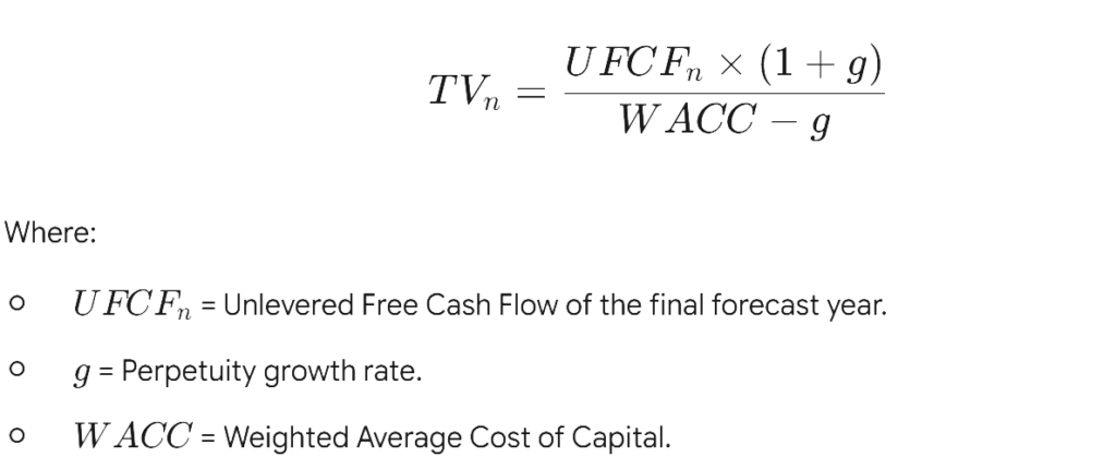
The Golden Rule of g
The perpetuity growth rate (g) cannot exceed the long-term growth rate of the economy. If you set g at 4% while the global GDP grows at 2.5%, your model mathematically implies that this single company will eventually swallow the entire world economy. In practice, g is typically benchmarked against long-term inflation (1.5% – 2.5%) or GDP growth (2% – 3%).
Method 2: The Exit Multiple Method
The Exit Multiple Method (EMM) is the weapon of choice in Private Equity. It assumes the business will be sold at the end of the forecast period to a strategic buyer or another financial sponsor.
The Formula
Instead of projecting cash flows to infinity, you apply an financial multiple (usually EV/EBITDA or EV/EBIT) to the financial metric of the final forecast year (n) or the forward year (n+1).
How to Find the Right Multiple
The multiple is derived from Comparable Companies Analysis (Comps) or Precedent Transactions. If similar mature companies in the sector are currently trading at 10x EBITDA, your exit multiple should generally hover around that range, often adjusted downwards to be conservative.
Exit Multiple Method vs Perpetuity Growth: Which One to Use?
| Feature | Gordon Growth Method (Perpetuity) | Exit Multiple Method (EMM) |
| Core Assumption | The company operates forever at a steady state. | The company is sold at the end of the horizon. |
| Best Used For | Mature, stable, cyclical, or asset-heavy businesses (e.g., Telecom, Energy). | High-growth companies, Tech, and Private Equity LBO models. |
| Pros | Theoretically sound; rooted in academic financial theory. | Highly practical; reflects current market realities and exit strategies. |
| Cons | Extremely sensitive to the WACC – g spread. | Market multiples fluctuate wildly based on the economic cycle. |
The Pro-Tip: Sanity Check Both
Never use one method in a vacuum. If you use the Exit Multiple Method, back-solve for the implied perpetuity growth rate to see if it makes sense.
If your 14x EBITDA exit multiple implies a 5.5% perpetuity growth rate, your multiple is too aggressive. Conversely, if your 2% growth rate implies a 4x EBITDA multiple for a software company, your valuation is likely too conservative.
How Not to Mess Up: 3 Fatal Terminal Value Mistakes
1. Forgetting the “Steady State” Check
You cannot transition into Terminal Value if your company hasn’t reached a steady state by Year 5. If your revenue is growing at 25% in Year 5, applying a 2% perpetuity growth rate in Year 6 creates a catastrophic drop-off that breaks the logic of the model. You either need to extend your discrete forecast period (e.g., to Year 10) or fade the growth rate gradually.
2. Misaligning CapEx and Depreciation
In the terminal period, a company cannot grow without investing. If your terminal growth rate (g) is 2%, your Capital Expenditures (CapEx) must be greater than or equal to Depreciation & Amortization (D&A) to support that growth. A common rookie mistake is leaving CapEx much lower than D&A in perpetuity, which artificially inflates the cash flows.
3. Blindly Trusting a Single Point Estimate
Because the TV has a disproportionate impact on Enterprise Value, presenting a single valuation number is a red flag. Always build a Sensitivity Table (Data Tables in Excel) crossing WACC vs. Perpetuity Growth Rate, or WACC vs. Exit Multiple.
Investment committees don’t look for a single “correct” number; they look for a defensible range of value.
Conclusion
Calculating the Terminal Value isn’t just about plugging numbers into the Gordon Growth formula or slapping an EBITDA multiple on Year 5. It requires a deep understanding of macroeconomic constraints, sector dynamics, and the long-term sustainability of the asset.
Next time you build a DCF, cross-check your methods, align your terminal CapEx, and ensure your implied growth rates don’t defy the laws of economics. Your investment committee will thank you.